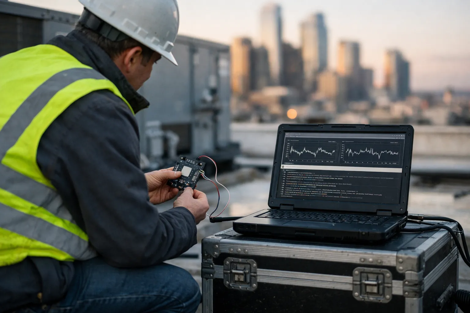
Rooftop packaged units (RTUs) remain workhorses of commercial HVAC fleets, yet many faults — stuck dampers, fouled filters, economizer failures, compressor cycling anomalies — go undetected until comfort complaints or energy waste appear. Edge fault detection and diagnostics (FDD) using TinyML (machine learning optimized for microcontrollers) offers a low-latency, privacy-preserving, and affordable path to continuous monitoring without moving every sensor stream to the cloud.
What this guide covers
- How to plan an edge FDD deployment for RTUs
- Sensor selection and sampling plans
- Feature engineering and labeling strategies
- Model selection, training, and quantization for TinyML
- Hardware options, secure integration, and commissioning checklist
- Operational maintenance, drift detection, and common pitfalls
Why TinyML at the edge?
Deploying lightweight models at the unit level reduces bandwidth, lowers latency for alarms, and keeps raw data local for privacy. Modern microcontrollers (ESP32-S3, RP2040, STM32) and single-board computers (Raspberry Pi Zero 2 W) can run quantized neural nets or classical models (decision trees, SVM) packaged with TensorFlow Lite Micro or optimized C libraries. For many RTU faults, models under 1 MB can achieve useful detection rates.
Step 1 — Define target faults and success metrics
Choose a limited set of high-value, detectable faults. Typical examples for RTUs:
- Stuck economizer damper (partial/fully stuck)
- Outdoor-enthalpy control failure (outdoor/return mixing wrong)
- Clogged return filter / reduced airflow
- Compressor short-cycling or failed staging
- Coil frost or low refrigerant charge (manifesting as low superheat or abnormal currents)
Establish metrics: detection latency (minutes), precision/recall (target F1>0.80 for initial models), false alarm rate per unit per month, and allowable compute footprint (e.g., 1 MB flash, 256 KB RAM).
Step 2 — Sensor selection and placement
Start with signals already available on the unit controller or the field wiring. Add sensors only when necessary.
- Temperature: supply air, return air (room), mixed-air, evaporator inlet/outlet. Use industrial 10 kΩ NTC or PT100/PT1000 for accuracy ±0.2–0.5°C.
- Pressure/flow: static pressure in supply plenum (pitot or differential sensor), duct static pressure to infer airflow drop.
- Current/power: CT on compressor and fan motors (split-core CTs) to detect staging and cycling.
- Actuator feedback: damper position (0–10 V or potentiometer), valve position sensors.
- Vibration acoustics (optional): MEMS accelerometer at motor or compressor for mechanical faults.
- Outdoor air conditions: temperature, humidity (for economizer mis-operation).
Sampling rate guidance: 0.2–1 Hz for temperature/flow/current is usually sufficient. For vibration or acoustic anomalies sample at 100–1,000 Hz but process on-device to extract features (RMS, spectral bands).
Step 3 — Data collection and labeling
Good models require labeled examples. Options:
- Historical operations: extract normal operation windows and known fault events from BAS logs and work orders.
- Targeted fault injection: during off-peak hours simulate stuck dampers, staged compressor disables, dirty filter (partial blockage) under controlled conditions. Ensure safety and document start/stop times.
- Synthetic augmentation: time-warp, noise injection, and controlled scaling for small datasets — helpful but never a substitute for real fault captures.
Collect at least several dozen fault instances of each class, and many more normal windows. Use a central store for labeling (CSV or time-series DB). Keep metadata: unit ID, ambient conditions, control setpoints, and technician note.
Step 4 — Feature engineering
On-device models benefit from compact, informative features. Compute these as rolling-window aggregates:
- Steady-state deltas: supply_temp - return_temp, mixed-air - outdoor_temp
- Control residuals: commanded_damper_pos - measured_pos, VFD_speed - inferred airflow
- Statistical features: mean, std, min/max, skew over 1–15 minute windows
- Derivative features: 1st and 2nd order differences to capture ramping and cycling
- Frequency-domain summaries (for vibration): band energy, spectral centroid
- Energy-normalized metrics: compressor current per ton (to detect low charge)
Keep feature vectors small (8–32 features) to limit model size. Normalize using rolling windows or unit-specific baselines (z-score). For edge deployments, precompute normalization parameters in training and store fixed scalers on-device, or periodically send scaler updates from the cloud.
Step 5 — Model selection and training
Two practical architectures:
- Classical ML: random forest or gradient-boosted trees (XGBoost) for server-side training and export to small decision trees for edge. Trees are interpretable and fast.
- Tiny neural nets: 1–2 hidden layers with small width, or 1D CNNs for sequence features. Convert to TensorFlow Lite and quantize to int8 for microcontrollers.
Training tips:
- Use stratified cross-validation. Guard against data leakage by splitting by unit and date.
- Address class imbalance with focal loss, class weights, or oversampling of faults.
- Optimize for operational metrics (precision at low false alarm rate) rather than raw accuracy.
- Profile model size and latency early: prefer models 256 KB binary and inference latency 200 ms on target MCU.
Step 6 — Quantization, pruning and TFLite Micro
Convert models to TensorFlow Lite format and quantize to 8-bit. Use TensorFlow Model Optimization Toolkit for pruning if necessary. For microcontrollers use TensorFlow Lite Micro (TFLM) to run models without an OS dependency. For slightly bigger hardware (Raspberry Pi Zero 2 W), standard TFLite with int8 and the Coral Edge TPU (USB) can accelerate inference.
Step 7 — Hardware choices and integration
Hardware options depend on model size and required I/O:
- Minimal MCU: ESP32-S3 (8–16 MB flash, ~400 KB usable RAM) — good for very small models and direct sensor interfacing (ADC, I2C, UART).
- More capable MCU: STM32H7 or RP2040 with external PSRAM — for slightly larger models and deterministic MCU RTOS stacks.
- Edge SBC: Raspberry Pi Zero 2 W — supports full Python/TFLite stacks, easier local logging and MQTT TLS, but consumes more power.
- Acceleration: Coral Edge TPU USB (paired with Pi) for larger quantized models with low latency.
Integration: expose alerts to BAS or facility dashboards via MQTT with TLS to a central broker (Mosquitto, managed MQTT), using a secure client certificate. Optionally publish summarized telemetry (feature aggregates and anomaly scores) to a time-series DB (InfluxDB) or analytics platform.
Step 8 — Commissioning checklist
- Verify sensor calibration and wiring; log initial baselines for 48–72 hours.
- Confirm sampling rates and feature computation on device; inspect values via serial or MQTT.
- Run model in parallel mode (silent) for 1–2 weeks to compare on-device scores with ground truth and server-side models.
- Tune thresholds to reach desired precision/recall trade-off; set escalation rules for alarms (e.g., anomaly must persist 10 minutes before alert).
- Enable secure OTA (code and model updates) with signature verification.
- Document alarm descriptions and recommended corrective actions for technicians.
Step 9 — Operations: maintenance and model lifecycle
Operational considerations:
- Monitor model drift: track prediction distributions and concept drift. If anomaly rates steadily increase or drop, collect labeled data and retrain.
- Scheduled retraining: every 3–6 months or after major equipment changes. Maintain a labeled dataset repository.
- False positives: create suppression windows (e.g., during maintenance) and route technician feedback back into labels.
- Security: rotate certificates, isolate devices on an HVAC VLAN, and log firmware/model changes for audit.
Example deployment metrics (realistic)
Sample small deployment: 50 RTUs, ESP32-S3 agents, 8 features sampled at 1 Hz aggregated into 60-second windows. Daily outbound telemetry (anomaly scores + feature summaries) per unit ~5–10 KB; peak daily uplink ~250–500 KB per unit. Initial model size 120 KB (int8), inference latency ~30 ms on ESP32-S3. Typical cost per unit: sensors & wiring $150–400, controller hardware $40–120, commissioning labor $250–600.
Common pitfalls and how to avoid them
- Pitfall: Too many fault classes initially — start with 2–4 high-value faults to prove ROI.
- Pitfall: Inadequate labels — plan fault injection or technician-assisted labeling during commissioning.
- Pitfall: Overly sensitive thresholds — tune to operational tolerance and use persistence windows to reduce nuisance alarms.
- Pitfall: Ignoring unit variance — normalize per-unit baselines or use unit ID as a model feature.
Resources & tools
- TensorFlow Lite Micro — compact runtime for MCUs
- Edge hardware: ESP32-S3, Raspberry Pi Zero 2 W, Coral USB Accelerator
- MQTT brokers: Mosquitto, HiveMQ
- Time-series stores: InfluxDB, TimescaleDB
- Visualization: Grafana, Node-RED dashboards
Final recommendations
Edge FDD using TinyML is a practical, cost-effective path to earlier detection of rooftop unit faults and measurable energy savings. Begin small, validate with real fault captures, and iterate: accurate detection requires good sensors, clear labeling, conservative commissioning thresholds, and an operational plan for retraining and technician feedback. With a deliberate rollout you can turn RTUs from passive devices into active contributors to reliability and decarbonization goals.