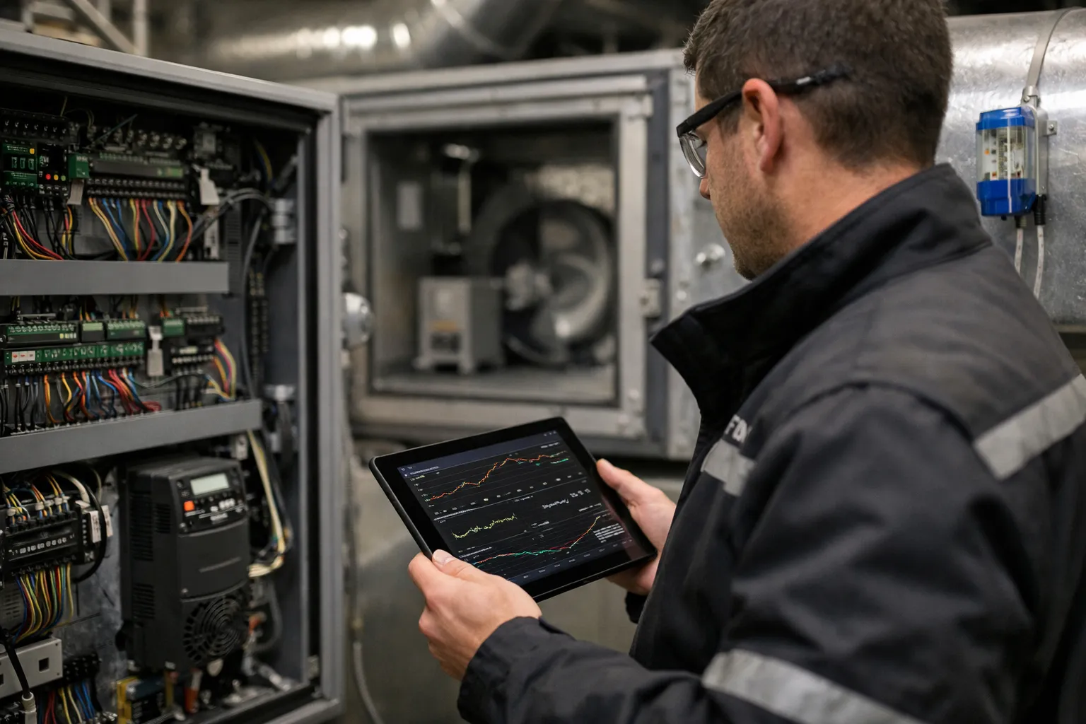
Precise control of air‑handling unit (AHU) loops—supply‑air temperature, duct static pressure, economizer position, and recirculation dampers—directly affects occupant comfort, energy use and equipment life. In 2026, building automation systems (BAS) from vendors such as Tridium Niagara 4, Siemens Desigo, Schneider EcoStruxure and Johnson Controls Metasys routinely include autotune and adaptive control features. But field technicians still need a rigorous manual commissioning workflow to verify sensors, actuators and tuning logic, and to capture reliable baseline data.
Scope and purpose
This guide walks you through a complete field commissioning and tuning process for PID control loops on AHUs. It is written for HVAC enthusiasts and field techs who want practical, repeatable steps: pre‑checks, data collection, tuning (autotune and manual), validation tests and documentation. It covers common loops (supply‑air temperature and duct static pressure) and control enhancements such as cascade, feedforward and anti‑windup. Wherever formulas are shown, units and assumptions are explicit—ensure you translate values to your controller’s scaling.
Before you begin: tools, timing and safety
- Schedule: Perform tuning during low‑occupancy hours (nights or weekends) to avoid comfort complaints and to allow the AHU to run through steady states.
- Personnel: Two‑person minimum—operator and a safety/observer who can isolate equipment if needed.
- Tools: BAS access (secure credentials), trend historian or datalogger (1‑Hz or faster preferred for dynamics), laptop/tablet with CSV export, clamp meter (VFD verification), differential manometer for duct static, calibrated temperature probes, portable power meter (optional).
- Safety: Lockout/tagout when working on hardware, establish emergency stop procedures for fans and dampers, and notify occupants and facilities managers of planned tests.
Step 1 — Pre‑commissioning checks
- Verify sensor calibrations: measure supply and return air temperatures, mixed air, and duct static with a calibrated probe to confirm BAS sensor offsets. Record offsets in the commissioning report.
- Confirm actuator health: stroke valves/dampers across their full range and verify travel times and end switches. Replace or repair noisy/slow actuators before tuning.
- Check mechanicals: belts, coils, filters and fan bearings should be in good condition—mechanical faults distort loop dynamics.
- Document control logic: obtain ladder or control sequence diagrams. Identify loop inputs and outputs, control mode (direct/reverse), output limits and interlocks.
- Set safe output limits: restrict VFD speed, valve positions, damper travel to safe ranges for testing.
Step 2 — Collect baseline data
Record steady states and dynamic responses before changing tuning:
- Export at least 30–60 minutes of baseline trends for the loop (setpoint, PV, controller output, actuator position, ambient conditions).
- Capture extremes: hottest/coldest supply air during normal operation and any existing oscillations.
- Document sample rate and time zone—high sample rates (1–10 s) make step response analysis easier.
Step 3 — Choose a tuning approach
There are three practical approaches:
- Autotune (BAS built‑in): Fast and convenient. Use when the controller’s autotune algorithm is proven on the platform and actuators are healthy. Always perform a manual verification afterward.
- Reaction‑curve (open‑loop) Ziegler–Nichols: Safe for processes you can step (change valve or fan speed) and measure the process reaction curve (dead time L and time constant T). Good when autotune is unavailable.
- Closed‑loop (ultimate gain) Ziegler–Nichols: Produces aggressive gains by finding the gain that causes sustained oscillation. Use with caution and only if safety limits and fast shutdown are available.
How to measure for the reaction‑curve method
- Put loop in manual and set controller output to a steady value (e.g., 30%).
- Apply a step change (e.g., raise output to 40% — a 10% step). Record the process variable (PV) response.
- From the PV step response, identify dead time L (time between step and first measurable PV response) and time constant T (time to reach 63.2% of the total change after L).
- Calculate process gain K: K = ΔPV / ΔMV (change in PV divided by change in manipulated variable — e.g., °F per % output).
Step 4 — Compute PID parameters (reaction‑curve Ziegler–Nichols)
For the reaction‑curve method the commonly used Ziegler–Nichols PID formulas are:
- Kc (controller gain) = 1.2 × (T / (K × L))
- Ti (integral time) = 2 × L
- Td (derivative time) = 0.5 × L
Notes: K is process gain in PV units per controller output unit (e.g., °F per %). Many controllers express proportional action as gain Kp or proportional band; be sure to convert formulas to your controller’s units.
Worked example (supply‑air temperature)
Scenario: A 10% increase in heating valve position raises supply air temperature by 3.0°F (so K = 3.0°F / 10% = 0.3 °F/%). From the step test you measure dead time L = 30 s and time constant T = 150 s.
- Compute Kc = 1.2 × (150 / (0.3 × 30)) = 1.2 × (150 / 9) = 1.2 × 16.67 ≈ 20 (% output per °F). That is, with 1°F error the controller output will change ~20%.
- Ti = 2 × 30 = 60 s
- Td = 0.5 × 30 = 15 s
Interpretation: If your controller accepts proportional gain (Kp) in units of % output per °F, enter Kp ≈20, Ti = 60 s, Td = 15 s. If it uses proportional band or different units, convert accordingly.
Step 5 — Conservative commissioning and validation
Ziegler–Nichols settings are intentionally aggressive for disturbance rejection. For occupied buildings, reduce Kc to 50–80% of the computed value and increase Ti by 20–50% to avoid oscillation. Follow this validation sequence:
- Apply the reduced gain and run the loop in closed loop with setpoint changes and disturbance simulations (e.g., damper position changes, VFD speed changes).
- Record PV, MV and controller output. Look for settling time, overshoot (>10% is usually unacceptable for comfort loops), and steady‑state error.
- If oscillation appears, reduce Kc further or increase Ti. If response is sluggish, increase Kc in small increments.
- Enable derivative (Td) sparingly—derivative can amplify noise. Use a low pass filter on derivative if available.
Advanced options: cascade, feedforward and anti‑windup
- Cascade control: Use an inner loop (e.g., valve position to coil outlet temperature) and an outer loop (supply air temperature). Tune inner loop first—its faster dynamics benefit outer loop stability.
- Feedforward: Add feedforward from outdoor air temperature or return air temperature to the SAT loop to reduce disturbance effects—particularly effective on economizers.
- Anti‑windup: Ensure integral anti‑windup is enabled to prevent integrator buildup during actuator saturation (valve fully open or closed, VFD maxed out).
Step 6 — Acceptance criteria and tests
Establish measurable acceptance tests and capture evidence (trends and CSV exports):
- Steady‑state error: within ±0.5°F for SAT loops; ±0.02 in. w.c. for duct static when achievable.
- Settling time: define target (for example, SAT loop returns to within 10% of setpoint change within X minutes—customize by system size).
- Overshoot: less than 10% for comfort loops; safety limits trip before dangerous overshoot.
- Robustness: loop remains stable under expected disturbances (filter loading, drafts, mixed‑air changes).
Document all tests, include raw trend files, and attach annotated graphs showing step tests and final tuned response.
Common pitfalls and troubleshooting
- Sensor drift: A biased sensor masks true dynamics—calibrate first.
- Actuator backlash and dead zones: Valve stiction or damper slop adds dead time—measure and repair where possible; compensatory tuning is limited.
- Interacting loops: Simultaneous tuning of interacting loops (e.g., SAT and duct static) can cause chasing—tune the fastest inner loop first and use cascade where appropriate.
- Noisy PV signal: Apply filtering in the controller or use a moving average—avoid heavy filtering that slows control response.
- Relying only on autotune: Autotune is a useful tool, but verify its results and don’t accept parameters blindly—review logs and perform manual step checks.
Handover, documentation and periodic review
Deliver a commissioning packet that includes:
- Baseline trends, step test CSVs and annotated plots
- Final PID values and controller scaling/units
- Acceptance test results and signed checklist
- Sensor calibration certificates and actuator travel records
- Recommendations for retune schedule (seasonal retunes are common: spring start and fall recomission for heating loops)
Recommend also enabling alarm monitoring for loop instability (oscillation detectors) and setting up a routine where trends are reviewed after major system changes (filter replacements, coil cleanings, or control upgrades).
When to call for advanced controls
In 2026 many BAS platforms include adaptive PID, model predictive control (MPC) and cloud‑based analytics. Use these when your building has multiple interacting plants, aggressive energy goals, or when persistent occupant comfort issues exist despite careful PID tuning. However, even with advanced controls, solid field data, calibrated sensors and verified actuator health remain prerequisites.
Final checklist (quick)
- Calibrate sensors and verify actuators.
- Collect and save baseline trends.
- Choose tuning method (autotune or manual reaction‑curve).
- Perform safe step tests, measure L, T and K.
- Compute PID values, apply conservatively and validate.
- Document tests, export trend files and sign acceptance tests.
- Schedule periodic reviews and set alarms for instability.
Well‑executed PID commissioning transforms AHU control from guesswork to predictable, energy‑efficient behavior. With good measurement, conservative application of tuning rules, and a disciplined validation and documentation workflow, field teams can deliver reliable comfort and measurable energy savings—while building the data set that enables more advanced controls in the future.